































Table of Contents
- Key Points
- Understanding Diffusion Models
- Leveraging the U-Net Architecture
- Diffusion Model: benefits and drawbacks
- FAQ
- Related Questions


Understanding Diffusion Models
Diffusion Models as Noise Removal Networks
At their core, diffusion models are designed to be powerful noise removal systems. Unlike other generative algorithms that try to directly predict an image, diffusion models work by progressively removing noise from a starting point of randomness. Think of it like taking a blurred, staticky TV screen and gradually tuning it until a clear image emerges.
To understand this better, let’s compare diffusion models to other generative neural networks like:
- Variational Autoencoders (VAEs): VAEs learn a compressed representation of the input data, called a latent space. New images can then be generated by sampling from this latent space and decoding it.
- Generative Adversarial Networks (GANs): GANs use two neural networks (a generator and a discriminator) to compete against each other, with the generator learning to create realistic images that fool the discriminator.
And yes, diffusions as well, input some random noise and convert them to an image.
While VAEs and GANs are also generative neural nets, diffusion models approach the image generation task differently, inputting some random noise and converting them to images. Instead of directly generating clean images, diffusion models learn to reverse a gradual process of adding noise.
If you're simply generating images without any prompts or conditions, it is called unconditional image generation. When you want to generate specific images, we train with prompts and label information; these are called conditional generative models.
This approach allows for greater control and flexibility in the image generation process.
To illustrate how diffusion models generate images, consider the following steps:
- A fully noisy image is taken, an image filled with nothing but random pixels.
- The Neural Network iteratively removes noise from the image.
- With enough noise removal, you can see a clear, realistic image.
Forward Diffusion: Adding Noise
The magic of diffusion models lies in two opposing processes: forward diffusion and reverse diffusion.
Forward diffusion, also known as the diffusion process, is a carefully crafted procedure of gradually adding noise to an initial image. This is done in discrete time steps, slowly degrading the image until it becomes indistinguishable from pure random noise.
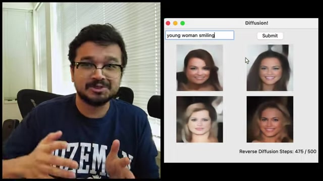
You can imagine this process like adding milk to water: the milk slowly diffuses into the water as time goes by, from being clear water at t=0 to pure white at t=N.
- T = 0: At the start, you have a clear image.
- T = N: At the end, you are left with only noise.
A key component of forward diffusion is the DDPM (Denoising Diffusion Probabilistic Models) scheduler. This scheduler defines how the noise is added at each time step. The DDPM scheduler uses number of steps, beta start and beta end parameters for the project.
Mathematically, each single step of noise addition can be added following a specific formula:
Xt = √(1 - βt) Xt-1 + √(βt) ε, where ε ~ N(0, I)
Where:
- Xt is the image at a timestamp t
- Xt-1 is the image at a previous timestamp
- ε represents Gaussian Noise
- βt represents the noise variance
But adding noise iteratively is inefficient, the authors use math to write Xt as a function of X0 to speed up the process. However this is for generating images and not competing with platforms like midjourney.
In a nutshell, the network can take a fully noisy image and iteratively remove the noise. The entire purpose of forward diffusion is to generate a dataset that the network can use to remove the noise.
Reverse Diffusion: Denoising and Image Generation
Now that we have polluted our pristine image to noise, the generative model needs to be able to revert the process. Reverse diffusion is the process of starting with purely random noise and learning to step-by-step remove the noise to get back to a coherent, realistic image.
The network is trained to predict the epsilon, and the network’s prediction is used to denoise the image, following an inverse of the equation that was previously stated

. The entire diffusion network is a de-noising network.
In terms of math, the network imports a noisy image at a timestamp and will be trained to output the noise. The function returns the noisy image at the input timestep.
The whole process can be done with a Neural Network and the help of the DDPM scheduler in order to progressively de-noise the image. This process requires the understanding of both forward and reverse diffusion, which is the key to understanding diffusion.
Leveraging the U-Net Architecture
The U-Net for Noise Prediction
A critical component of many diffusion models is the U-Net architecture. This architecture consists of encoder and decoder block. Downsampling through convolutional layers progressively decreases the image resolution. At the final step of the network a fully de-noised images will be shown.
The power of UNet is that it can combine both shallow features of the image alongside deep features to properly show an image in its final stage. To help the UNet models even further, time step embeddings are introduced, providing more information about how close the model is from getting the final image, it's a small token of acknowledgement to what has been done to the image.








Most people like


































Report
Please select a reason for reporting
- 13 Reasons to Switch from Snapchat to Text Messaging
- 7 Powerful Speech to Text Apps to Boost Productivity
- 10 Best Speech to Text Tools for Effortless Transcription
- 13 Free Tools to Easily Transcribe Audio to Text
- 15 Surprising Ways Google's Speech-to-Text Boosts Productivity
- 7 Best Free Online Audio to Text Transcription Tools
- 9 Tips to Transcribe Speech to Text Faster and Better
- 13 Best Speech to Text Software for Windows 10 in 2023
- 7 Tips for Choosing the Best Transcriber for Audio to Text
- 11 Reasons Why Dragon Speech-to-Text Apps are Game-Changers
- 6 Secrets to Enhance Your Speech to Text Transcription
- 6 Brilliant Ways to Boost Productivity with Talk-to-Text on Your MacBook
- 6 Ways Transcription Software Converts Audio to Text
- 8 Tips to Transcribe Speech to Text Like a Pro
- 6 Reasons IBM Watson Speech to Text is a Game-Changer
- 14 Powerful Ways Talk-to-Text Improves Your Workflow
- 12 Top Windows Speech-to-Text Software for Efficient Transcription
- 12 Game-Changing Benefits of Apple's Speech to Text Technology
- 9 Powerful Use Cases for AWS Speech to Text Technology
- 10 Easy Steps to Transcribe YouTube Videos to Text
- transcription audio en texte
- online audio transcription
- free audio file transcription
- free ai audio transcription
- audio transcription service
- audio transcription online free
- audio transcription free online
- audio to transcription software
- audio and transcript
- ai audio transcription free
- voice recording to text converter
- translate voice recording to text
- record voice to text
- audio recording to text converter
- voice recording and transcription
- chatgpt voice to text
- gmail voice to text
- speech to text reader
- speech to text ai free
- speech to talk
- How SEO and Marketing Dashboards Empower Agencies to Drive Results
- How to Use AI Tools to Find Internal Linking Opportunities Across a Business Website
- Discover Your Perfect Haircut with AI Hairstyle Apps
- Free Reputation Calculator Tools: How They're Adapting to Score AI Visibility, Not Just Rankings
- Design Professional Flyers for Free on Your Phone
- Best Free Flyer Maker Apps for Android: Design Like a Pro
- How to Know If Your Business Is Ready for an AI Customer Service Agent
- Revolutionizing Storytelling: From Novels to Screenplays with AI
- Create Engaging Animated Explainer Videos with a Free AI Tool
- Stop Multi-Subscribing: Benchmark Top AI Visual Models in One Canvas
- ASOMobile Helps Teams Benchmark App Store Screenshots Against Competitors
- How to Match LMS Software With Your Organization's Training Plan
- Revolutionizing Email Marketing Agency with AI
- How to Convert BTC to HNT
- Unleashing the Power of AI: Cognizant's Roadmap for Transformation
- Frame to Video Review: A Practical Look at Turning Two Still Frames Into Motion
- NVIDIA NIM: Revolutionizing Supply Chain Data Analysis with AI
- Top AI Tools That Help Brands Stand Out Offline (Not Just Online)
- Top 5 Cold Email Software: Maximize Your Outreach in 2025
- Magic School AI: Revolutionizing Quiz & Assessment Generation

Copyright ©2026 toolify