































Table of Contents
- Key Points
- Excel Interview Test: Questions and Solutions
- Advanced Excel Techniques for Data Analysis
- Step-by-Step Guide: Conditional Formatting in Excel
- Frequently Asked Questions
- Related Questions



Excel Interview Test: Questions and Solutions
Question 1: Highlight the 10 Lowest Orders in Red
The first question
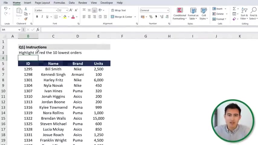
is a straightforward task designed to assess your familiarity with conditional formatting. The goal is to highlight the 10 lowest order values in a given dataset in red. This is a common task in data analysis, as it allows you to quickly identify outliers or key metrics.
To achieve this, start by selecting the range of cells containing the order values. Then, navigate to the Home tab in Excel, and click on Conditional Formatting. From the dropdown menu, choose Top/Bottom Rules and then select Bottom 10 Items.
A dialog box will appear, allowing you to customize the formatting. Ensure that the number 10 is entered, and choose the desired formatting style – in this case, Light Red Fill with Dark Red Text. Click OK, and Excel will automatically highlight the 10 lowest order values in red.
For a quick way to select cells, use the shortcut Ctrl+Shift+Down Arrow after selecting the first cell in the data column.
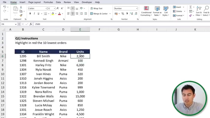
This selects data to the bottom to apply the formatting to all the data.
Question 2: Accept or Reject Projects Based on Minimum Requirements Using IF and AND
This question requires you to use an IF statement with an AND condition to determine whether projects should be accepted or rejected based on minimum revenue and profit requirements. It tests your ability to make logical decisions within Excel.
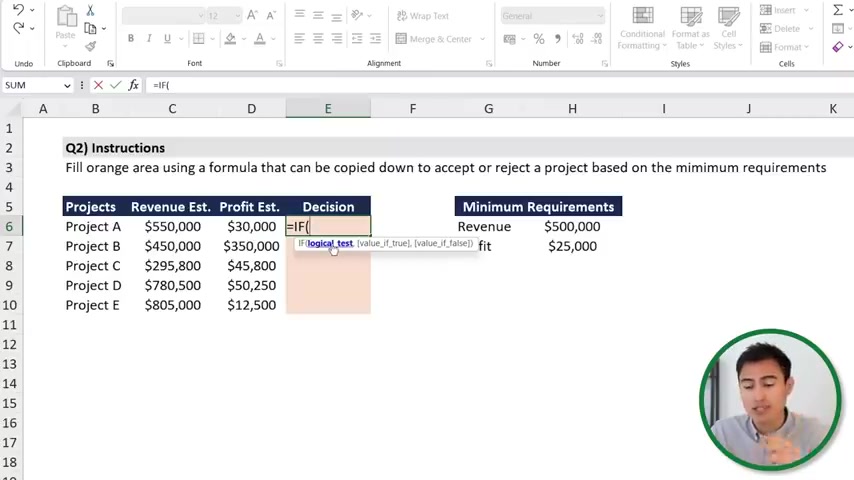
The instructions ask to fill the orange area using a formula that can be copied down to accept or reject a project based on the minimum requirements.
First, you'll need to use the IF function combined with the AND function. The AND function lets you evaluate multiple conditions. For each project, you'll check if both the revenue and profit exceed the minimum requirements. If both conditions are true, the project is accepted; otherwise, it's rejected.
The formula will look something like this:
=IF(AND(Revenue >= MinimumRevenue, Profit >= MinimumProfit), "Accept", "Reject")Replace Revenue and Profit with the appropriate cell references for each project's revenue and profit. Replace MinimumRevenue and MinimumProfit with the cells containing the minimum revenue and profit requirements. It's also essential to lock the minimum revenue and profit with the F4 key to ensure when the formulas are dragged down the correct criteria are still used. This formula will return “Accept” if both the revenue and profit figures meet the criteria.
Remember to drag the formula down to apply it to all projects in the dataset.





Most people like







































Report
Please select a reason for reporting
- 13 Reasons to Switch from Snapchat to Text Messaging
- 7 Powerful Speech to Text Apps to Boost Productivity
- 10 Best Speech to Text Tools for Effortless Transcription
- 13 Free Tools to Easily Transcribe Audio to Text
- 15 Surprising Ways Google's Speech-to-Text Boosts Productivity
- 7 Best Free Online Audio to Text Transcription Tools
- 9 Tips to Transcribe Speech to Text Faster and Better
- 13 Best Speech to Text Software for Windows 10 in 2023
- 7 Tips for Choosing the Best Transcriber for Audio to Text
- 11 Reasons Why Dragon Speech-to-Text Apps are Game-Changers
- 6 Secrets to Enhance Your Speech to Text Transcription
- 6 Brilliant Ways to Boost Productivity with Talk-to-Text on Your MacBook
- 6 Ways Transcription Software Converts Audio to Text
- 8 Tips to Transcribe Speech to Text Like a Pro
- 6 Reasons IBM Watson Speech to Text is a Game-Changer
- 14 Powerful Ways Talk-to-Text Improves Your Workflow
- 12 Top Windows Speech-to-Text Software for Efficient Transcription
- 12 Game-Changing Benefits of Apple's Speech to Text Technology
- 9 Powerful Use Cases for AWS Speech to Text Technology
- 10 Easy Steps to Transcribe YouTube Videos to Text
- transcription audio en texte
- online audio transcription
- free audio file transcription
- free ai audio transcription
- audio transcription service
- audio transcription online free
- audio transcription free online
- audio to transcription software
- audio and transcript
- ai audio transcription free
- voice recording to text converter
- translate voice recording to text
- record voice to text
- audio recording to text converter
- voice recording and transcription
- chatgpt voice to text
- gmail voice to text
- speech to text reader
- speech to text ai free
- speech to talk
- How SEO and Marketing Dashboards Empower Agencies to Drive Results
- How to Use AI Tools to Find Internal Linking Opportunities Across a Business Website
- Discover Your Perfect Haircut with AI Hairstyle Apps
- Free Reputation Calculator Tools: How They're Adapting to Score AI Visibility, Not Just Rankings
- Design Professional Flyers for Free on Your Phone
- Best Free Flyer Maker Apps for Android: Design Like a Pro
- How to Know If Your Business Is Ready for an AI Customer Service Agent
- Revolutionizing Storytelling: From Novels to Screenplays with AI
- Create Engaging Animated Explainer Videos with a Free AI Tool
- Stop Multi-Subscribing: Benchmark Top AI Visual Models in One Canvas
- Magic School AI: Revolutionizing Quiz & Assessment Generation
- Create Your Own Email Bot and Automate Your Email Tasks
- Beyond Pure Prompts: Optimizing Production with 'Text With Reference' Generation
- Stop Using Boring TTS: My Honest Deep Dive Into VideoAI and the Hunt for the Perfect Custom Voices
- AI & Elections: Defending Democracy Against Misinformation
- Navigating Political Discourse: AI, Deepfakes, and Reality Checks
- Detecting Political Bias in News Articles: A Powerful AI Algorithm
- AI Bias Unveiled: Political Leanings in ChatGPT & Beyond
- Revolutionize Learning: Discover Quizzes AI for Engaging Interactive Quizzes
- From AI-Generated to Audience-Ready: How Quillbot Humanize AI Is Changing the Content Editing Process

Copyright ©2026 toolify