































Table of Contents
- Key Points
- Graphing Exponential Equations: The Fundamentals
- Transforming Exponential Equations into Logarithmic Form
- Step-by-Step Graphing Exponential Equations
- Tools Needed for Graphing Exponential Functions
- Exploring the Upsides and Downsides of Exponential Functions
- FAQ
- Related Questions


Graphing Exponential Equations: The Fundamentals
What is an Exponential Function?
An exponential function is a mathematical function where the independent variable (x) appears in the exponent. It generally takes the form of y = a^x, where 'a' is the base and 'x' is the exponent.
This fundamental understanding sets the stage for graphing these equations. Exponential functions are characterized by rapid growth or decay, depending on whether the base 'a' is greater than 1 or between 0 and 1.
Before diving into graphing, it's essential to understand the components that define exponential functions. This primarily includes understanding the constant ratio, the zero term and the use of negative exponent rules. The constant ratio helps define the rate at which the function grows.
These properties are crucial for not only graphing exponential functions but also for understanding their impact in real-world scenarios, such as population growth, compound interest, and radioactive decay. Let’s explore the domain and range of exponential functions, along with specific restrictions, to build a solid foundation before we start graphing.
Understanding Domain and Range
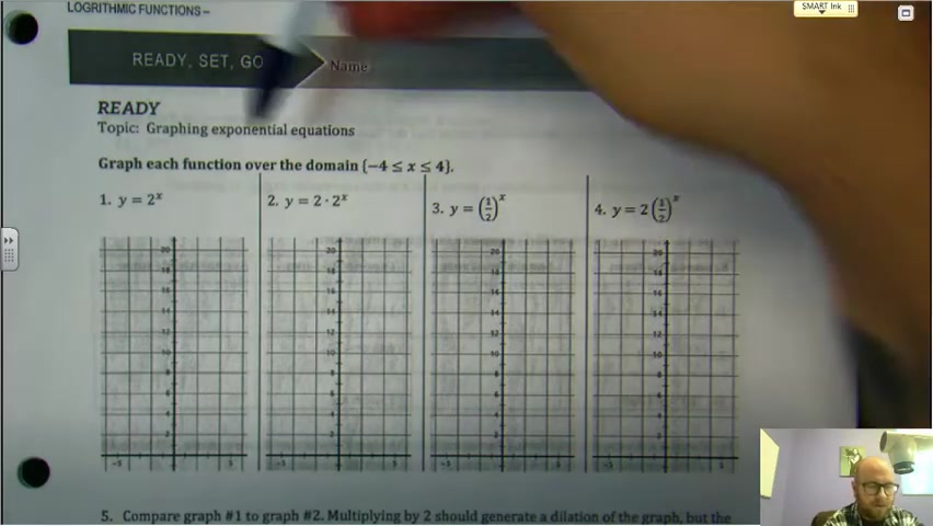
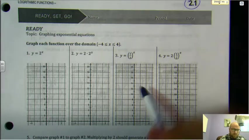
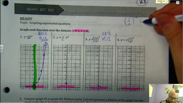
The domain of an exponential function typically includes all real numbers. However, for practical graphing purposes, it's often necessary to limit the domain to a specific range. For instance, if you're instructed to graph the function over the domain -4 ≤ x ≤ 4, you’ll only consider x-values within this interval.
The range of an exponential function, on the other hand, is usually all positive real numbers, excluding zero. This is because any number raised to any power will never result in zero or a negative number, given a positive base. Understanding these domain and range constraints helps in accurately plotting the function and interpreting its behavior. Now, let’s examine the general form of an exponential equation to dissect its components and how they influence the graph.
The General Form of Exponential Equations
The general form of an exponential equation is given by: *y = n₀ CR^x**
Where:
- y: The dependent variable
- n₀: The initial value or the y-intercept (where x = 0)
- CR: The constant ratio, also known as the growth or decay factor
- x: The independent variable
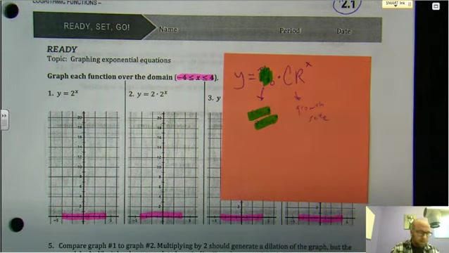
The initial value (n₀) is the starting point on the y-axis. The constant ratio (CR) determines the rate at which the function grows or decays. A constant ratio greater than 1 indicates growth, while a constant ratio between 0 and 1 indicates decay. To illustrate this, consider the equation y = 2^x. Here, the initial value is 1 (since any number multiplied by an implied 1 at the start) and the constant ratio is 2, signifying exponential growth. Now, let's proceed to graph a basic exponential function.
Transforming Exponential Equations into Logarithmic Form
Understanding the Logarithmic Form
Exponential functions and logarithms are intimately related. Understanding this connection can be very helpful. The logarithmic form is expressed as y = logₐ(x), which reads as "y equals the logarithm base a of x." This form is equivalent to the exponential form x = a^y.
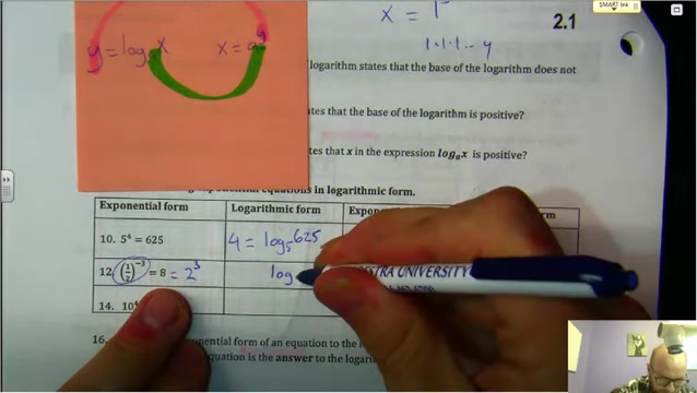
The key is to recognize that a logarithm answers the question, “To what power must 'a' be raised to equal 'x'?” Therefore, understanding this relationship allows you to switch between exponential and logarithmic forms seamlessly. Now, let's explore the significance of key components within exponential and logarithmic definitions.
Understanding Crucial Logarithmic and Exponential Definitions
Several crucial definitions must be kept in mind. This includes: that the base of a logarithm cannot be equal to one and also, a base of log must be positive
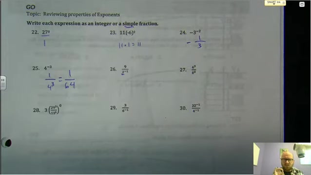
*   The base of the logarithm can’t be 1 because 1 raised to any power is always 1, making the logarithm undefined.
*   The base needs to be positive to avoid complex numbers and ensure a consistent domain.
Let’s put what you’ve learned to the test with some practice exercises. From simple graphing, to understanding the general form of the equations and to transforming the function. Now let's see how all of these techniques can make graphing and resolving equations a cinch.
Step-by-Step Graphing Exponential Equations
Graphing y = 2^x
To graph y = 2^x over the domain -4 ≤ x ≤ 4, you need to calculate the corresponding y-values for each x-value in the domain.
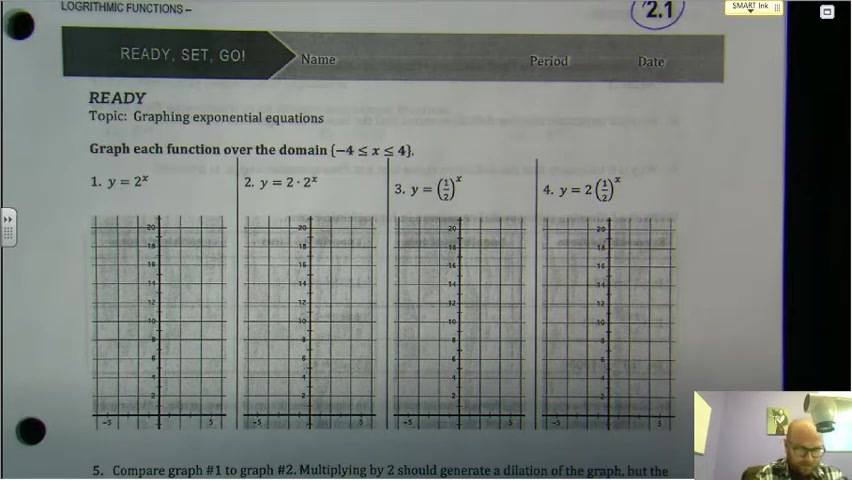
This involves simple substituion with each negative number from the stated domain having to be converted to its inverse before resolving
Here’s how you can do it:
| x | y = 2^x |
|---|---|
| -4 | 2^(-4) = 1/16 |
| -3 | 2^(-3) = 1/8 |
| -2 | 2^(-2) = 1/4 |
| -1 | 2^(-1) = 1/2 |
| 0 | 2^(0) = 1 |
| 1 | 2^(1) = 2 |
| 2 | 2^(2) = 4 |
| 3 | 2^(3) = 8 |
| 4 | 2^(4) = 16 |
Plot these points on a graph. Notice the exponential increase as x becomes more positive. The graph starts very close to the x-axis for negative x-values, gradually rising and then rapidly increasing. Remember to only draw the graph within the specified domain (-4 to 4). This will give you the curve of an exponential function with a starting value of 1 and a constant ratio of 2. Now, let's explore how multiplying the exponential equation by a constant affects the graph’s dilation.
Compare Graph #1 to Graph #2
When an exponential equation is multiplied by a constant, such as changing from y = 2^x to y = 2 * 2^x, the graph undergoes a vertical dilation.
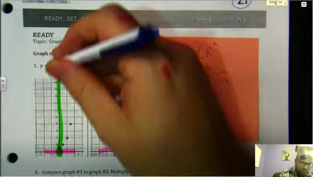
This multiplication stretches the graph along the y-axis, making the function grow (or decay) more rapidly. In practice, each y-value of the original graph is multiplied by the constant, effectively altering the scale but not the fundamental shape of the exponential curve.
Now, let’s shift gears and look at exponential decay, where the base 'a' in y = a^x is a fraction between 0 and 1. This change has significant implications for the graph’s direction.
Graphing Exponential Decay: y = (1/2)^x
Exponential decay occurs when the base of the exponential function is between 0 and 1.
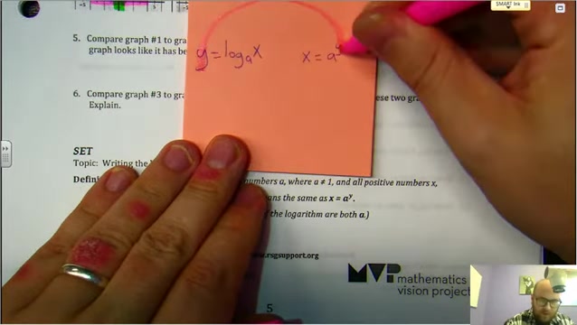
For example, consider the equation y = (1/2)^x. As x increases, y decreases, approaching the x-axis but never touching it.
To graph this, calculate y-values for several x-values within the domain -4 ≤ x ≤ 4:
| x | y = (1/2)^x |
|---|---|
| -4 | (1/2)^(-4) = 16 |
| -3 | (1/2)^(-3) = 8 |
| -2 | (1/2)^(-2) = 4 |
| -1 | (1/2)^(-1) = 2 |
| 0 | (1/2)^(0) = 1 |
| 1 | (1/2)^(1) = 1/2 |
| 2 | (1/2)^(2) = 1/4 |
| 3 | (1/2)^(3) = 1/8 |
| 4 | (1/2)^(4) = 1/16 |
Plot these points, and you'll observe that as x increases positively, the function decays towards the x-axis, starting from higher y-values for negative x. Now, let’s address handling negative exponents to accurately graph exponential equations.
Working with Negative Exponents
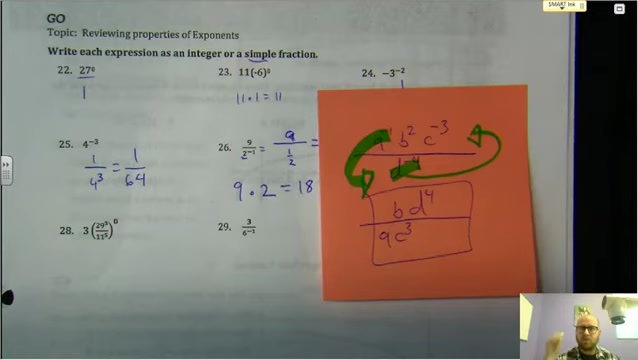
Negative exponents indicate inverse operations.
When you encounter a negative exponent, you need to take the reciprocal of the base. For instance, in the equation y = 2^(-x), each y-value is the reciprocal of what it would be for y = 2^x at the same x-value. Thus, to graph exponential functions accurately, handling negative exponents correctly is paramount. With these graphing techniques in hand, we can Translate exponential functions into logarithmic forms.
Tools Needed for Graphing Exponential Functions
Essentials for Effective Graphing
While graphing exponential functions, several key tools can be highly beneficial:
- Graph Paper: Provides a structured grid for accurate plotting.
- Pencils and Erasers: Allows for precise drawing and easy corrections.
- Graphing Calculator: Simplifies the evaluation of exponential functions and provides quick visualization.
- Online Graphing Tools (Desmos, GeoGebra): Offers interactive, dynamic graphing experiences.
With these tools at your disposal, you can tackle graphing exponential equations with greater confidence and precision.






Most people like





























Report
Please select a reason for reporting
- 13 Reasons to Switch from Snapchat to Text Messaging
- 7 Powerful Speech to Text Apps to Boost Productivity
- 10 Best Speech to Text Tools for Effortless Transcription
- 13 Free Tools to Easily Transcribe Audio to Text
- 15 Surprising Ways Google's Speech-to-Text Boosts Productivity
- 7 Best Free Online Audio to Text Transcription Tools
- 9 Tips to Transcribe Speech to Text Faster and Better
- 13 Best Speech to Text Software for Windows 10 in 2023
- 7 Tips for Choosing the Best Transcriber for Audio to Text
- 11 Reasons Why Dragon Speech-to-Text Apps are Game-Changers
- 6 Secrets to Enhance Your Speech to Text Transcription
- 6 Brilliant Ways to Boost Productivity with Talk-to-Text on Your MacBook
- 6 Ways Transcription Software Converts Audio to Text
- 8 Tips to Transcribe Speech to Text Like a Pro
- 6 Reasons IBM Watson Speech to Text is a Game-Changer
- 14 Powerful Ways Talk-to-Text Improves Your Workflow
- 12 Top Windows Speech-to-Text Software for Efficient Transcription
- 12 Game-Changing Benefits of Apple's Speech to Text Technology
- 9 Powerful Use Cases for AWS Speech to Text Technology
- 10 Easy Steps to Transcribe YouTube Videos to Text
- transcription audio en texte
- online audio transcription
- free audio file transcription
- free ai audio transcription
- audio transcription service
- audio transcription online free
- audio transcription free online
- audio to transcription software
- audio and transcript
- ai audio transcription free
- voice recording to text converter
- translate voice recording to text
- record voice to text
- audio recording to text converter
- voice recording and transcription
- chatgpt voice to text
- gmail voice to text
- speech to text reader
- speech to text ai free
- speech to talk
- Design Professional Flyers for Free on Your Phone
- Best Free Flyer Maker Apps for Android: Design Like a Pro
- How to Know If Your Business Is Ready for an AI Customer Service Agent
- Revolutionizing Storytelling: From Novels to Screenplays with AI
- Create Engaging Animated Explainer Videos with a Free AI Tool
- Stop Multi-Subscribing: Benchmark Top AI Visual Models in One Canvas
- Best Seedance 2.5 API Provider: Every Price on the Market, Checked at Source
- AI OnlyFans: How to Generate $30,000/Month (Legally)
- Transform Your Script into an Engaging Video with AI Video Maker!
- AI Marketing Automation: A Comprehensive Guide for Small Businesses
- Design Professional Flyers for Free on Your Phone
- Best Free Flyer Maker Apps for Android: Design Like a Pro
- Unleash Creativity: AI Coloring Pages with ColoringBook.ai
- Generate Stunning AI Photos with Google Gemini: A Guide
- Boost Your Etsy Sales with Stunning Digital Invitations!
- Revolutionize Your Etsy Listing with AI Text Generator
- Create Coloring Pages with AI: A Bing AI Tutorial
- Photo Lab App: Transform Your Photos with Stunning AI Effects
- Effortless Design: Rewriting Text with Microsoft Designer's AI
- Create & Sell Kids' Coloring Books with AI - KDP Guide

Copyright ©2026 toolify