Laplacian Gaussian Edge Detection: Techniques & Implementation

In the realm of computer vision, edge detection plays a pivotal role in image analysis and understanding. Among the various edge detection techniques, the Laplacian of Gaussian (LoG) stands out for its ability to effectively reduce noise while accurately identifying edges. This article delves into the intricacies of the LoG technique, exploring its principles, implementation, and practical applications.

What is Laplacian Gaussian (LoG)?

The Laplacian of Gaussian (LoG) is a second-order derivative edge detector that combines the Laplacian operator with a Gaussian filter.

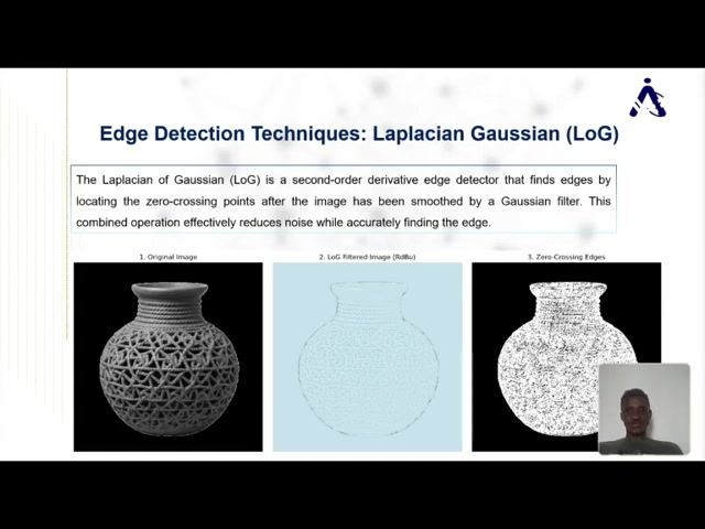
The Laplacian operator is sensitive to noise, so the Gaussian filter is used to smooth the image before applying the Laplacian. This combined operation effectively reduces noise while accurately finding edges. LoG helps find edges by locating the zero-crossing points after the image has been smoothed. In simpler terms, think of the LoG as a way to blur an image slightly and then sharply highlight the boundaries, effectively reducing the impact of imperfections and focusing on the essential shapes. It is a process critical in applications like medical imaging and object recognition where precision is key. This technique is particularly effective when dealing with images that are inherently noisy, ensuring that the detected edges are genuine features rather than artifacts of the noise.

The Math Behind LoG

The LoG operation involves convolving an image with the LoG kernel, which is the Laplacian of the Gaussian function. The Gaussian function is defined as:

$$G(x, y) = \frac{1}{2\pi\sigma^2} e^{-\frac{x^2 + y^2}{2\sigma^2}}$$

where $$\sigma$$ is the standard deviation of the Gaussian distribution.

The Laplacian operator is defined as:

$$ abla^2 f = \frac{\partial^2 f}{\partial x^2} + \frac{\partial^2 f}{\partial y^2}$$

The LoG kernel is then the Laplacian of the Gaussian function:

$$LoG(x, y) = abla^2 G(x, y) = -\frac{1}{\pi\sigma^4} \left[ 1 - \frac{x^2 + y^2}{2\sigma^2} \right] e^{-\frac{x^2 + y^2}{2\sigma^2}}$$

Convolution: The LoG kernel is convolved with the image. Convolution involves sliding the LoG kernel over the image, multiplying the kernel values by the corresponding image pixel values, and summing the results to produce a new pixel value in the output image. This process is repeated for every pixel in the image, resulting in a filtered image that highlights regions of rapid intensity change.

Zero-Crossing Detection: After the convolution, the zero crossings in the filtered image are detected. These zero crossings correspond to the edges in the original image. The LoG operator is particularly useful in edge detection because it efficiently combines noise reduction (through the Gaussian filter) and edge enhancement (through the Laplacian operator).

Benefits of Using LoG in Edge Detection

Noise Reduction: The Gaussian filter component of LoG smooths the image, reducing the impact of noise on edge detection. This ensures that the identified edges are more likely to be real features rather than noise artifacts.

Edge Enhancement: The Laplacian operator enhances edges by highlighting areas of rapid intensity change. This sharpens the edges, making them more distinct and easier to detect.

Isotropic Response: LoG exhibits an isotropic response, meaning that it detects edges equally well regardless of their orientation. This is important for applications where edges may occur in any direction.

Single Operator: LoG combines smoothing and differentiation into a single operator, simplifying the edge detection process. This reduces the complexity of the algorithm and makes it more efficient to implement.

Setting Up the Environment

Before diving into the code, ensure you have the necessary libraries installed. For this implementation, we will primarily use OpenCV (cv2) and NumPy.

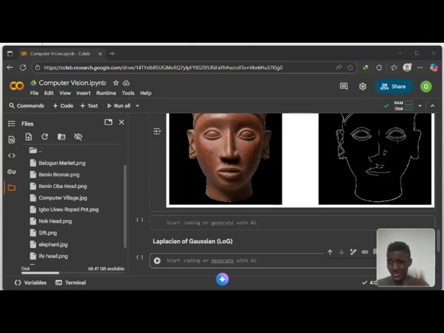
These are standard libraries for image processing and numerical computations in Python.

pip install opencv-python numpy

Once these libraries are installed, you can import them into your Python environment.

import cv2
import numpy as np
import matplotlib.pyplot as plt

Implementing LoG in Python with OpenCV

Here's the Python code to implement LoG edge detection using OpenCV:

def laplacian_of_gaussian(image, kernel_size, sigma):
    """Applies the Laplacian of Gaussian filter to an image.

    Args:
        image (numpy.ndarray): The input image.
        kernel_size (int): The size of the Gaussian kernel.
        sigma (float): The standard deviation of the Gaussian kernel.

    Returns:
        numpy.ndarray: The LoG filtered image.
    """
    # Apply Gaussian blur
    blurred = cv2.GaussianBlur(image, (kernel_size, kernel_size), sigma)

    # Apply Laplacian operator
    log = cv2.Laplacian(blurred, cv2.CV_64F)

    return log

# Load the image [t:01:17]
image = cv2.imread('Igbo Ukwu Roped Pot.png', cv2.IMREAD_GRAYSCALE)

# Define the parameters [t:01:17]
kernel_size = 5
sigma = 1.4

# Apply the LoG filter [t:01:49]
log_image = laplacian_of_gaussian(image, kernel_size, sigma)

# Display the original and LoG filtered images [t:01:49]
plt.figure(figsize=(12, 6))

plt.subplot(1, 2, 1)
plt.imshow(image, cmap='gray')
plt.title('Original Image')
plt.axis('off')

plt.subplot(1, 2, 2)
plt.imshow(log_image, cmap='gray')
plt.title('Laplacian of Gaussian')
plt.axis('off')

plt.show()

Code Explanation

• laplacian_of_gaussian(image, kernel_size, sigma) function: This function takes the input image, kernel size, and standard deviation as arguments and applies the LoG filter.

• cv2.GaussianBlur(image, (kernel_size, kernel_size), sigma): Applies a Gaussian blur to the image using the specified kernel size and standard deviation.

• cv2.Laplacian(blurred, cv2.CV_64F): Applies the Laplacian operator to the blurred image. The cv2.CV_64F argument specifies that the output image should have a 64-bit floating-point data type to handle negative values.

• plt.imshow(image, cmap='gray'): Displays the original and LoG filtered images using Matplotlib.

• plt.axis('off'): Turns off the axes for a cleaner display.

Understanding the parameters

The parameters used in the LoG implementation are crucial for achieving optimal results.

• kernel_size: This parameter defines the size of the Gaussian kernel. A larger kernel size results in more blurring, which can be useful for reducing noise but may also blur important details.
• sigma: This parameter defines the standard deviation of the Gaussian kernel. It controls the amount of blurring applied to the image. A larger sigma results in more blurring.

The table below summarizes the key parameters:

Additional Considerations

Data Type: The cv2.CV_64F data type is used to ensure that the Laplacian operator can handle negative values. This is important for accurately detecting edges.

Zero-Crossing Detection: The code provided only applies the LoG filter. To complete the edge detection process, you would need to implement zero-crossing detection.

Thresholding: Thresholding can be used to further refine the edge detection results by removing weak or spurious edges. This involves setting a minimum intensity value below which edges are discarded.

Implementing Zero-Crossing Detection

To detect zero crossings, you can iterate through the LoG filtered image and check the sign of neighboring pixels. If there is a change in sign, it indicates a zero crossing and thus an edge.

def detect_zero_crossings(image):
    """Detects zero crossings in an image.

    Args:
        image (numpy.ndarray): The input image.

    Returns:
        numpy.ndarray: A binary image indicating the zero crossings.
    """
    # Create an output image
    zero_crossings = np.zeros_like(image)

    # Iterate through the image
    for i in range(1, image.shape[0] - 1):
        for j in range(1, image.shape[1] - 1):
            # Check for zero crossings
            if (image[i-1, j] * image[i+1, j] < 0) or \
               (image[i, j-1] * image[i, j+1] < 0) or \
               (image[i-1, j-1] * image[i+1, j+1] < 0) or \
               (image[i+1, j-1] * image[i-1, j+1] < 0):
                zero_crossings[i, j] = 255
    return zero_crossings

# Apply zero-crossing detection
zero_crossings = detect_zero_crossings(log_image)

# Display the zero-crossing image
plt.imshow(zero_crossings, cmap='gray')
plt.title('Zero-Crossings')
plt.axis('off')
plt.show()

Enhancing Results with Parameter Adjustments

The quality of LoG edge detection hinges significantly on fine-tuning parameters such as kernel_size and sigma. Adjusting these parameters allows for a better balance between noise reduction and edge preservation.

1. Experiment with Different Kernel Sizes: Varying the kernel_size impacts the degree of blurring applied to the image. Larger kernels offer increased noise reduction but can also blur finer details. Smaller kernels preserve more detail but are more susceptible to noise. testing a range of values helps identify the optimal setting for specific image characteristics.
2. Tune the Sigma Value: The sigma value, representing the standard deviation, directly influences the Gaussian blur's intensity. Higher sigma values produce more aggressive blurring, ideal for highly noisy images, while lower values maintain image sharpness but may fail to adequately suppress noise.

By iteratively adjusting these parameters and visually assessing the edge detection results, users can tailor the LoG filter to match the unique challenges presented by their images, achieving enhanced edge detection performance.