































Table of Contents
- Key Points
- Basics of Computation Graphs
- Illustrative Example: A Simple Function
- Step-by-Step Forward Pass
- Cost Function Optimization
- Pros and Cons of Computation Graphs
- Frequently Asked Questions
- Related Questions



Basics of Computation Graphs
What is a Computation Graph?
A computation graph is a directed graph that represents the mathematical computations performed in a neural network. It helps Visualize how the data flows through the network during the forward and backward passes. Understanding computation graphs is fundamental to grasping how gradients are calculated and how backpropagation works. The graph organizes the computation into a series of nodes, where each node represents an operation, and edges represent the flow of data. This structured representation provides a clear path for both calculating the output and computing derivatives for optimization.

The organization using this way will be explained by computation graph. The computation graphs are useful for understanding why the forward pass and backward pass is the most efficient way to organize. The efficiency and clear visualization made it a very useful way to compute function.
Forward and Backward Passes
In neural networks, computation is typically divided into two phases: the forward pass and the backward pass. The forward pass involves feeding the input data through the network to compute the output. Each layer performs a series of operations, transforming the input data step by step until the final output is obtained.

This is the step to compute the output of the neural network. Then following by a backward pass, which calculates the gradients. The backward pass, or backpropagation, computes the gradients of the cost function with respect to the network's parameters. These gradients are then used to update the parameters during training, helping the network learn. The backward pass leverages the chain rule of calculus to efficiently compute these gradients layer by layer. The gradients calculation is important since the gradients are important to compute derivatives. Derivatives is a key element for machine learning and computation graph explains its organization.
Illustrative Example: A Simple Function
Defining the Function J(a, b, c)
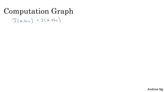
To illustrate the concept of a computation graph, let's consider a simple function: J(a, b, c) = 3 (a + b c). This function takes three variables, a, b, and c, as inputs and performs a series of arithmetic operations to produce a single output, J. This function is far more simple than using logistic regression or the complicated neural network. The example is meant to show how computation graph can explain the process. To compute this function, we can break it down into a series of distinct steps
:
- Compute u = b * c
- Compute v = a + u
- Compute J = 3 * v
By breaking down the computation into smaller steps, we can easily represent it using a computation graph.
Constructing the Computation Graph
The computation graph for our function J(a, b, c) consists of nodes representing the inputs (a, b, c) and the intermediate variables (u, v), as well as the final output (J). The edges between the nodes represent the flow of data and the operations performed. This step is very important since it is the process of constructing a computation graph. To construct a graph with the function specified above. We can first write a,b,c. And followed by the output of the function.
The computation graph is constructed as follows:
- Inputs: a, b, c
- Intermediate Variable 1: u = b
- c
- Intermediate Variable 2: v = a + u
- Output: J = 3
- v
This graph visually represents the steps involved in computing the function J, providing a clear understanding of the computational process.
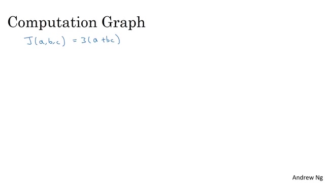
u = b * c, by the equation we store the variable as u. Then V = a + u which u can be brought from the previous steps. Finally the last output J = 3v. With this the computation is complete and ready to go into the final output.
A Concrete Numerical Example
To further illustrate the computation graph, let's consider a concrete numerical example. Suppose we have the following values:
- a = 5
- b = 3
- c = 2
Using these values, we can Trace the forward pass through the computation graph:
- u = b
- c = 3
- 2 = 6
- v = a + u = 5 + 6 = 11
- J = 3
- v = 3
- 11 = 33
Thus, the output of the function J(a, b, c) is 33 for these specific input values. This step helps to concrete to the variable since it provides numerical value for each operation.
This is important for understanding the value of J which is 3v. We can verify this steps to follow the equation so we will end up 33 as the value. It is calculated in this way: J(a,b,c) = 3(5 + 3 * 2) to get to 33 as final output.





Most people like






































Report
Please select a reason for reporting
- 13 Reasons to Switch from Snapchat to Text Messaging
- 7 Powerful Speech to Text Apps to Boost Productivity
- 10 Best Speech to Text Tools for Effortless Transcription
- 13 Free Tools to Easily Transcribe Audio to Text
- 15 Surprising Ways Google's Speech-to-Text Boosts Productivity
- 7 Best Free Online Audio to Text Transcription Tools
- 9 Tips to Transcribe Speech to Text Faster and Better
- 13 Best Speech to Text Software for Windows 10 in 2023
- 7 Tips for Choosing the Best Transcriber for Audio to Text
- 11 Reasons Why Dragon Speech-to-Text Apps are Game-Changers
- 6 Secrets to Enhance Your Speech to Text Transcription
- 6 Brilliant Ways to Boost Productivity with Talk-to-Text on Your MacBook
- 6 Ways Transcription Software Converts Audio to Text
- 8 Tips to Transcribe Speech to Text Like a Pro
- 6 Reasons IBM Watson Speech to Text is a Game-Changer
- 14 Powerful Ways Talk-to-Text Improves Your Workflow
- 12 Top Windows Speech-to-Text Software for Efficient Transcription
- 12 Game-Changing Benefits of Apple's Speech to Text Technology
- 9 Powerful Use Cases for AWS Speech to Text Technology
- 10 Easy Steps to Transcribe YouTube Videos to Text
- transcription audio en texte
- online audio transcription
- free audio file transcription
- free ai audio transcription
- audio transcription service
- audio transcription online free
- audio transcription free online
- audio to transcription software
- audio and transcript
- ai audio transcription free
- voice recording to text converter
- translate voice recording to text
- record voice to text
- audio recording to text converter
- voice recording and transcription
- chatgpt voice to text
- gmail voice to text
- speech to text reader
- speech to text ai free
- speech to talk
- Meshy AI: How to Create 3D Models from Text and Images
- How SEO and Marketing Dashboards Empower Agencies to Drive Results
- How to Use AI Tools to Find Internal Linking Opportunities Across a Business Website
- Discover Your Perfect Haircut with AI Hairstyle Apps
- Free Reputation Calculator Tools: How They're Adapting to Score AI Visibility, Not Just Rankings
- Design Professional Flyers for Free on Your Phone
- Best Free Flyer Maker Apps for Android: Design Like a Pro
- How to Know If Your Business Is Ready for an AI Customer Service Agent
- Revolutionizing Storytelling: From Novels to Screenplays with AI
- Create Engaging Animated Explainer Videos with a Free AI Tool
- Meshy AI: How to Create 3D Models from Text and Images
- ASOMobile Helps Teams Benchmark App Store Screenshots Against Competitors
- How to Match LMS Software With Your Organization's Training Plan
- Revolutionizing Email Marketing Agency with AI
- How to Convert BTC to HNT
- Unleashing the Power of AI: Cognizant's Roadmap for Transformation
- Frame to Video Review: A Practical Look at Turning Two Still Frames Into Motion
- NVIDIA NIM: Revolutionizing Supply Chain Data Analysis with AI
- Top AI Tools That Help Brands Stand Out Offline (Not Just Online)
- Top 5 Cold Email Software: Maximize Your Outreach in 2025

Copyright ©2026 toolify